New Publication: Power-law distribution in the number of confirmed COVID-19 cases

I just posted a new study on arXiv (see also this tweet) in which I study macro-epidemiological patterns in the COVID-19 pandemic and find that the distribution of confirmed cases in different countries follows a power-law distribution. In this post I will explain in simple terms what's the whole idea behind these ‘power-laws’ in COVID-19 prevalence and why I find it so interesting.

Background: huge variability in reported COVID-19 cases

With the ongoing corona-crisis, in the last weeks a huge number of theoretical studies on COVID-19 were made public. Most of these focused on time series analysis and mathematical modeling of case numbers, often in connection to intervention measures and the prediction of healthcare demand. In contrast, not many studies have addressed the biogeography of COVID-19. This is astonishing, as one of the striking characteristics of the pandemic is the huge variation in the number of cases that have been reported from different parts of the world. As of April 2020, some few countries, the so-called ‘epi-centers’ of the pandemics, were already severely struck by the pandemic, whereas many others at the same time had just confirmed the first few cases. Thus, while seeing dramatic scenes in the media, many people (still) experienced a mild number of cases in their local neighborhood. With my study I aim to quantify this phenomenon and provide some mechanistic explanation for this large geographic variability in COVID-19 prevalence.

There are some obvious explanations that come immediately to mind: A first possibility would be that the variation is caused by the idiosyncratic circumstances of the individual countries which differ largely in their geography and population size, but also in the way they are combatting the disease. Alternatively, parts of the variation could simply be due to reporting errors, reflecting disparate national testing regimes, with countries (e.g., China, South Korea, or Germany) having high testing rates, in contrast to other countries with much poorer testing. In my study, I argue, however, that a dominant part of this variation may be a direct consequence of the dynamics of the spreading process itself. Thereby, the epidemic prevalence in a country should be directly correlated to the arrival time of the disease: countries that were invaded very early by the virus have accumulated many cases in time, while countries with a late invasion naturally still have smaller prevalence.

Computing the distribution of COVID-19 prevalence

To investigate this further I computed the distribution of confirmed cases in different countries. For this I used the data from COVID-19 repository, operated by the Johns Hopkins University Center for Systems Science and Engineering (JHU CSSE). The database contains information about the daily number of confirmed COVID-19 cases and confirmed deaths in various countries worldwide.

The following figure shows the resulting histogram of the number of cases in different countries that have been reported on 22 March, 2020. 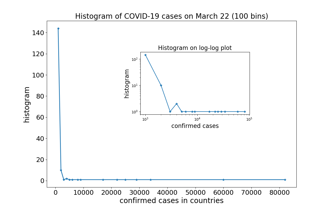The figure shows that the distribution is very broad. On that date, 168 countries were already invaded by the coronavirus. Thereby, the number of confirmed cases varied between 81,435 cases in China, followed by 59,138 cases in Italy, and so on, down to 1 case in 16 countries. This information is visualized in the histogram, which basically tells us that we have a very small number of countries with more than several thousand cases and a large number of countries with much fewer cases. This confirms our observation of an enormous variability in prevalence, as state above, but it does not provide much more insights. Obviously, the histogram is too broad (we say it has a long tail) to yield much information when plotted in this way.

This leads to the idea to plot the histogram with double-logarithmic axes (shown in the inset). However, despite using 100 bins for the 168 data points (corresponding to the 168 countries invaded by the virus at that date), the histogram still is very poorly resolved. What is needed is a way to obtain a histogram that resolves the case distribution both for small and large case numbers.

Histogram with logarithmic binning

A well-established solution is to sample the histogram with variable sized bins. This is shown the next figure, where I used bins at positions of powers of two (2,4,8,16, etc). This yields a histogram with bin positions that are equally spaced on a logarithmic scale. Such a histogram, however, would be unfair in the sense that larger bins naturally can ‘collect’ more counts. Therefore, in order to obtain a true probability distribution, the histogram counts must be normalized by the bin size, yielding the following plot of the COVID-19 case distribution P(n) in countries on a double logarithmic plot. 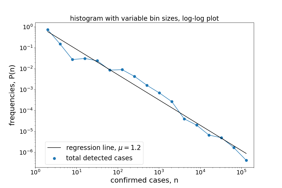The figure shows that the distribution of confirmed cases very closely follows a straight line on the double logarithmic plot. Very similar results can be found for the number of confirmed deaths. Note, that in my study on arXiv I used a slightly different method, where I made a histogram of log-transformed values and then used a back-transformed to obtain the distribution of non-logarithmic case numbers. Both methods, however, yield very similar results.

To illustrate the robustness of my hypothesis to spatial scale, I made the same analysis for confirmed COVID-19 cases in counties in the US. The next figure shows the corresponding distribution for the situation on 5 April, 2020. At this date 2,444 US counties were invaded by the virus. The largest epidemic prevalence was reported in New York City with 67,551 confirmed cases, while at the same time 359 counties only had a single confirmed case. 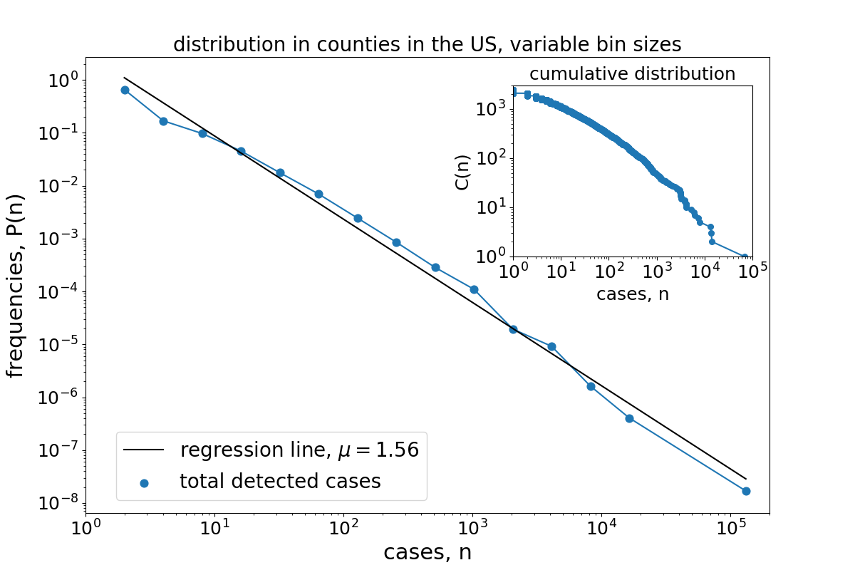Again the distribution P(n) closely follows a straight line on a double logrithmic plot. Thus, although the two data sets (cases in countries and US counties) differ greatly in spatial scale and resolution we obtain very similar prevalence patterns, confirming the robustness of the analysis.

Another way to represent the variability of case numbers is by plotting the cumulative distribution (shown in the inset of this figure), that is, the number C(n) of counties that have a number of confirmed cases larger than n. Also the cumulative distribution roughly resembles a straight line on the double logarithmic plot, even though a slight curvature of the line is clearly visible.

Power-law distributions are scale free

The fact that the distribution P(n) of COVID-19 cases, both in countries worldwide and in counties in the US, follows a straight line on a double logarithmic plots, expresses that fact the distribution can be described as a power-law

This simple law accurately describes the distribution over five orders of magnitude, from the largest case number to n=1, the minimal value of the power-law distributiona (for more information on this topic I recommend this excellent review by Mark Newman).

Using this distribution we can now quantify the huge variability of COVID-19 cases more precisely. The bulk of the distribution occurs for the many countries (or US counties) with a small number of confirmed cases. In contrast, there are a few countries with numbers of confirmed cases that are much higher than the typical value - the epi-centers of the pandemic, producing the long tail to the right of the distribution. The remarkable fact now is that there is a smooth transition from the left of the distribution (the many countries with few cases) to the right of the distribution (the few countries with many cases). Along this transition with every increase in case numbers we obtain a reduction in the number of corresponding countries - and this reduction is the the same at all scales!

This scale-free property is the hallmark of a power-law distribution. It allows allows to express the whole distribution with a single number, the critical exponent $\mu$, and it is a strong indication that the case numbers worldwide are governed by a common process.

Inequality of COVID-19 case and the 90/10 rule

From the slope of the regression line we can obtain a rough estimate of the critical exponent of the power-law, yielding a value of about $\mu=1.2$ for the country distribution and about $\mu=1.55$ for the US county distribution. Note, there are much better ways to estimate the critical exponents (as explained in my study). In both cases, the critical exponent is well below 2 which is remarkable as this value is unusally small, indicating a distribution without a defined mean.

The occurrence of a power-law with such a small critical exponent indicates an extraordinary inequality of the distribution. This can be quantified by calculating the fraction of the total number of confirmed cases in dependence of the fraction of the most affected countries (the so-called Lorenz curve). For the case of the COVID-19 distribution on 22 March, 95.7% of confirmed cases had been reported in the 20% most affected countries. Similarly, 90% of all confirmed cases had accumulated in the top 10% most affected countries and 82% of all confirmed cases had accumulated in the top 5% most affected countries. With 81,435 out of 336,953 confirmed cases on that day China alone had accumulated a fraction of 24% of all cases. The two most affected countries, China and Italy, together had accumulated a fraction of 41% of the worldwide reported cases.

Such numbers are frequently called the Pareto principle or 80/20 rule which states that for many systems roughly 80% of the effects come from 20% of the causes. For example, the richest 20% of the world's population roughly combine 80% of the world's income. In the case of the COVID-19 distribution we find that this imbalance is much larger, probably better described as a 90/10 rule. In fact, for a critical exponent of $\mu < 2$ we would theoretically expect that in the limit of an infinite sample size all cases should appear in a single country.

Caution when dealing with power-laws

When experienced scientists from statistical physics or complex sciences see a posting about a new power-law finding, some warning bells immediately goes off. This is due to a large history of questionable studies involving power-law distributions.

A dual scale process

We can explain the emergence of the power-law distribution with the following simple theory.